PYTHON程式語言的學習-numpy

import numpy as np

1. 建立陣列
產生指定陣列，或是從原本的list跟shape (tuple)更改。a.shape是

import numpy as np # 建立一維陣列 a = np.array([1,2,3]) print(a) print('a.shape=',a.shape) # 建立二維陣列 b = np.array([[1,2,3,4], [5,6,7,8], [9,10,11,12]]) print(b) print('b.shape=',b.shape,type(b.shape)) #將list換成numpy array: km_list = [3, 5, 10, 21, 4.5] km_array = np.array(km_list) print(km_array) #產生3*2，裡面數值皆為0的陣列 A=np.zeros((3,2)) print(A) #產生3*5，裡面數值皆為1的陣列 B=np.ones((3,5)) print(B)

[1 2 3] a.shape= (3,) [[ 1 2 3 4] [ 5 6 7 8] [ 9 10 11 12]] b.shape= (3, 4) [ 3. 5. 10. 21. 4.5] [[0. 0.] [0. 0.] [0. 0.]] [[1. 1. 1. 1. 1.] [1. 1. 1. 1. 1.] [1. 1. 1. 1. 1.]]




---



2. 產生指定數字範圍的陣列：np.arange(起始,結束)

import numpy as np #產生數字範圍 arr1 = np.arange(10) #從0到9 print(arr1) arr2 = np.arange(3,11) print(arr2) arr3 = np.arange(4,12,2) print(arr3)

[0 1 2 3 4 5 6 7 8 9] [ 3 4 5 6 7 8 9 10] [ 4 6 8 10]




---



3. 產生填滿指定數字的陣列: np.full((the shape),the value)
如果我們想要創其他數值的話，可以使用np.full((the shpae),the value)。語法full_like(陣列名稱, 數值）

c=np.full((3,3),99) print(c) a = np.array([[1,2,3,4,5,6,7],[7,6,5,4,3,2,1]]) b=np.full_like(a, 5) print('a=\n',a) print('b=\n',b)

[[99 99 99] [99 99 99] [99 99 99]] a= [[1 2 3 4 5 6 7] [7 6 5 4 3 2 1]] b= [[5 5 5 5 5 5 5] [5 5 5 5 5 5 5]]




---



4. 產生隨機陣列

import numpy as np np.random.seed(10) a1=np.random.rand(4) print('a1=',a1) a2=np.random.rand(3,2) print('a2=\n',a2) shape=(2,4) a3=np.random.rand(shape[0],shape[1]) print('a3=\n',a3) arr = np.random.rand(2,2) print(arr)

a1= [0.77132064 0.02075195 0.63364823 0.74880388] a2= [[0.49850701 0.22479665] [0.19806286 0.76053071] [0.16911084 0.08833981]] a3= [[0.68535982 0.95339335 0.00394827 0.51219226] [0.81262096 0.61252607 0.72175532 0.29187607]] [[0.91777412 0.71457578] [0.54254437 0.14217005]]




---




5. a.shape vs. a.ndim

import numpy as np # 建立一維陣列 a = np.array([1,2,3]) print(a) print('a.shape=',a.shape,type(a.shape)) print('a.ndim=',a.ndim) # 建立二維陣列 b = np.array([[1,2,3,4], [5,6,7,8], [9,10,11,12]]) print(b) # s=b.shape是b陣列的行列大小3*4，s=(3,4)=元組=tuple。 print('b.shape=',b.shape,type(b.shape)) print('b.ndim=',b.ndim) #將list換成numpy array: km_list = [3, 5, 10, 21, 4.5] km_array = np.array(km_list) print(km_array) #產生3*2，裡面數值皆為0的陣列 A=np.zeros((3,2)) print(A) #產生3*5，裡面數值皆為1的陣列 B=np.ones((3,5)) print(B) C=np.zeros((2,3,4)) print('C=\n',C) print(C.ndim)

[1 2 3] a.shape= (3,) a.ndim= 1 [[ 1 2 3 4] [ 5 6 7 8] [ 9 10 11 12]] b.shape= (3, 4) b.ndim= 2 [ 3. 5. 10. 21. 4.5] [[0. 0.] [0. 0.] [0. 0.]] [[1. 1. 1. 1. 1.] [1. 1. 1. 1. 1.] [1. 1. 1. 1. 1.]] C= [[[0. 0. 0. 0.] [0. 0. 0. 0.] [0. 0. 0. 0.]] [[0. 0. 0. 0.] [0. 0. 0. 0.] [0. 0. 0. 0.]]]




---




6. 改變陣列維度：a.reshape()

np1 = np.array([1, 2, 3, 4, 5, 6]) print('np1=',np1) print(np1[2]) np2 = np1.reshape([2, 3]) print('np2=',np2) print(np2[1, 0],np2[0,2]) np3 = np2.reshape([3, 2]) print('np3=',np3) print(np3[0, 1],np3[1, 0],np3[2,1])

np1= [1 2 3 4 5 6] 3 np2= [[1 2 3] [4 5 6]] 4 3 np3= [[1 2] [3 4] [5 6]] 2 3 6

---

before = np.array([[1,2,3,4],[5,6,7,8]]) print(before) after1 = before.reshape((8)) print(after1) after2 = after1.reshape((8,1)) print(after2) after3 = after2.reshape((2,4)) print(after3)

[[1 2 3 4] [5 6 7 8]] [1 2 3 4 5 6 7 8] [[1] [2] [3] [4] [5] [6] [7] [8]] [[1 2 3 4] [5 6 7 8]]




---



7. 陣列有什麼用？
陣列也就是數學上的矩陣有什麼用呢？同學們未來學量子物理的時候，就會明白基本上量子力學的數學架構就是要做矩陣的運算，包括計算矩陣的本徵值和本徵態，或者要利用矩陣來做向量的線性變換。物理系的學生最擅長的量子力學，也是未來高科技最重要的應用領域，所以同學們不用太早懷疑學這些有什麼用？它就是有很有用。雖然我們沒有辦法一下跳到三年級的課程，但是我們在下面會來介紹陣列的其他應用，特別是1維的陣列可以用來畫圖，二維和二維和三維的陣列可以用來儲存一張圖片，這都是我們在後續的課程中要大量應用的領域。

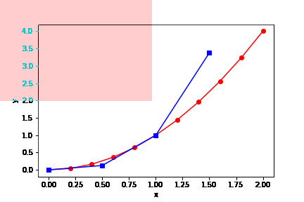
如果我們要畫一個函數所對應的圖形，首先一步就是要選擇一個畫圖的x區間\((a,b)\)，然後在這個區間中均勻地分割取點，再對這些\(x\)的點計算其對應的函數值y坐標，然後就可以對\((x,y)\)的數對來畫圖。numpy提供兩個好用的函數：np.linspace(a,b,N) and np.arange(a,b,dx)。 np.linspace(a,b,N) \(\rightarrow\) 在數值a和b的區間中分成N個點，a,b均包含在內。
np.arange(a,b,dx) \(\rightarrow\) 在數值a和b的區間中dx為分割的寬度，b不包含在內。


import matplotlib import matplotlib.pyplot as plt matplotlib.use("Agg") import numpy as np x = np.linspace(0,2,11) y = x**2 x2 = np.arange(0,2,0.5) y2 = x2**3 print('x=',x) print('y=',y) print('x2=',x2) print('y2=',y2) plt.figure() plt.xlabel('x') plt.ylabel('y') plt.plot(x,y,'r-o') plt.plot(x2,y2,'b-s') plt.savefig("fx-2.png") print ('plot is done')

x= [0. 0.2 0.4 0.6 0.8 1. 1.2 1.4 1.6 1.8 2. ] y= [0. 0.04 0.16 0.36 0.64 1. 1.44 1.96 2.56 3.24 4. ] x2= [0. 0.5 1. 1.5] y2= [0. 0.125 1. 3.375] plot is done




---



8. 更多的numpy範例程式
對已定義的矩陣做運算



import numpy as np a1 = np.arange(10) a2=a1**2 print(a1) print(a2) a = np.array([1,2,3,4]) b = np.array([10,20,30,40]) c = a + b ; print (c) c = a - b ; print (c) c = a * b ; print (c) c = a / b ; print (c)

[0 1 2 3 4 5 6 7 8 9] [ 0 1 4 9 16 25 36 49 64 81] [11 22 33 44] [ -9 -18 -27 -36] [ 10 40 90 160] [0.1 0.1 0.1 0.1]




---


np.identity(); 定義單位矩陣



a=np.identity(5) b=np.array([[1., 0., 0., 0., 0.], [0., 1., 0., 0., 0.], [0., 0., 1., 0., 0.], [0., 0., 0., 1., 0.], [0., 0., 0., 0., 1.]]) print('a=\n',a) print('b=\n',b)

a= [[1. 0. 0. 0. 0.] [0. 1. 0. 0. 0.] [0. 0. 1. 0. 0.] [0. 0. 0. 1. 0.] [0. 0. 0. 0. 1.]] b= [[1. 0. 0. 0. 0.] [0. 1. 0. 0. 0.] [0. 0. 1. 0. 0.] [0. 0. 0. 1. 0.] [0. 0. 0. 0. 1.]]




---


np.empty(); np.zeros(); np.ones(); np.full()



import numpy as np a1=np.empty((8)); print(a1) a2=np.zeros((8)); print(a2) a3=np.ones((8)); print(a3) for i in range(8): a3[i] = i print(a3) a4=np.full((8),9); print(a4)

[6.23042070e-307 4.67296746e-307 1.69121096e-306 8.45595292e-307 6.23058028e-307 2.22526399e-307 6.23053614e-307 7.56592338e-307] [0. 0. 0. 0. 0. 0. 0. 0.] [1. 1. 1. 1. 1. 1. 1. 1.] [0. 1. 2. 3. 4. 5. 6. 7.] [9 9 9 9 9 9 9 9]




---




import cv2 import numpy as np img = cv2.imread('fx-2.png') print(type(img)) print(img.shape) (Lx,Ly)=(img.shape[0],img.shape[1]) print('Lx=',Lx,' Ly=',Ly) Lx2=int(Lx/2); Ly2=int(Ly/2) for i in range(0,Lx): for j in range(0,Ly): if(i < Lx2 and j < Ly2): img[i][j][0]-=50;img[i][j][1]-=50;img[i][j][2]+=0 cv2.imwrite('fx-2B.png', img) print('done')

(288, 432, 3) Lx= 288 Ly= 432 done




---




9. 列表(list)運算和矩陣(array)運算的比較

   在下面的程式中所計算的內容是將兩個系列的數字(a,b)取它的平方和，計算的過程全部都寫成函數副程式來進行，並且這兩個函數副程式所使用的系列變數分別列表(def pySum)另外一個使用陣列(def npSum)。兩種運算方式都得到相同的結果。也請同學們藉由這個例子複習一下列表list它的用法，包括列表長度(len(a))和附加列表元素(c.append())的各種指令。並且也要複習函數副程式的寫法，副程式如何回傳資料，在主程式如何呼叫副程式。

def pySum():
    a = list(range(10))
    b = list(range(10))
    c = []
    for i in range(len(a)):
        c.append(a[i]**2 + b[i]**2)
    return c
c=pySum()
print(type(c))
print(c)

import numpy as np
def npSum():
    a = np.arange(10)
    b = np.arange(10)
    c = a**2 + b**2
    return c
c=npSum()
print(type(c))
print(c)

============output=============

[0, 2, 8, 18, 32, 50, 72, 98, 128, 162]

[  0   2   8  18  32  50  72  98 128 162]
>>> 

10. 比較兩種計算方法所花費的計算機時間

既然這兩種方法都可以得到相同的結果，我們為什麼有這兩種選項呢？一個很重要的原因，就是用np陣列所花費的計算機時間比列表所花的時間少許多，我們可以透過查詢計算機執行時間的指令來做比較。查詢計算機執行時間需要import time，執行的指令是time.time()。分別在兩個副程式的執行前和執行後都放上這個time.time()的指令，就可以測量該副程式執行的時間，再將兩個副程式所執行的時間相除就可以得到他們相對執行時間的倍率。為了放大執行的時間，我們將平方和的計算做了100000次。針對這個實際的例子我們不難發現用np陣列計算的速度比列表計算快了37倍，這主要是因為np陣列的計算程序用到向量的乘法，這是最簡單的一種平行計算方法。

import time
def pySum():
    a = list(range(100000))
    b = list(range(100000))
    c = []
    for i in range(len(a)):
        c.append(a[i]**2 + b[i]**2)
    return c

start1 = time.time()
c=pySum()
end1 = time.time()
T1=end1 - start1
print('CPU time using python list:',T1)


import time
import numpy as np
def npSum():
    a = np.arange(100000)
    b = np.arange(100000)
    c = a**2 + b**2
    return c

start2 = time.time()
c=npSum()
end2 = time.time()
T2=end2 - start2
print('CPU time using numpy array:',T2)
print('the ratio=', T1/T2)

============output=============
CPU time using python list: 1.2793054580688477
CPU time using numpy array: 0.03417539596557617
the ratio= 37.43352262421342
>>>