numpy是一個非常有用的數值計算工具,在這個講次中我們先簡單介紹矩陣的定義方法和基本的操作。
建立陣列1A
import numpy as np
a=np.full((5), 9)
print(a)
b=np.full((3,5), 4)
print(b)
print(a.shape)  # 矩陣的維度與大小
print(b.shape)
[9 9 9 9 9]
[[4 4 4 4 4]
 [4 4 4 4 4]
 [4 4 4 4 4]]
(5,)
(3, 5)
建立陣列1B
import numpy as np
x = np.array([1, 2, 3])
L =[1,2,3]
print ('x=',x)
print ('L=',L)
print ('請注意陣列array和列表list在輸出形式上的不同')
print (type(x), type(L))
y = np.arange(10)  # 類似 Python 的 range, 但是回傳 array
print ('y=',y)
z = np.arange(10,20,2)  #建立一個array,在10與20的之間以2的長度為間隔
print ('z=',z)
w = np.linspace(10,20,5) #建立一個array,在10與20之間5個點等分
print ('w=',w)
============輸出:=============
x= [1 2 3]
L= [1, 2, 3]
請注意陣列array和列表list在輸出形式上的不同

y= [0 1 2 3 4 5 6 7 8 9]
z= [10 12 14 16 18]
w= [10.  12.5 15.  17.5 20. ]
-
建立陣列2
在這個程式中我們引入2維和3維的陣列,並且使用shape指令來查詢陣列的維度和大小。
import numpy as np
a = np.array([1, 2, 3])   # 產生一維陣列
print(type(a))            # Prints ""
print(a.shape)            # 矩陣的維度與大小(1維且有3個元素)
print(a[0], a[1], a[2])   # 取出矩陣元素的寫法
a[0] = 5                  # 改變一個矩陣元素
print('a=',a)                  # 一個矩陣元素改變了
b = np.array([[1,2,3],[4,5,6]])    # 產生2維陣列
print('b=',b)
print(b.shape)                     # 矩陣的維度與大小(1維且有3個元素)
print(b[0, 0], b[0, 1], b[1, 0],b[1,2])  #取出矩陣元素的寫法,請注意對應關係
c=np.array([[[1,2,3],[4,5,6],[7,8,9]],[[2,2,3],[4,5,6],[7,8,9]]])
print('c=',c)
print(c.shape)
============output=============

(3,)
1 2 3
a= [5 2 3]
b= [[1 2 3]
 [4 5 6]]
(2, 3)
1 2 4 6
c= [[[1 2 3]
  [4 5 6]
  [7 8 9]]
 [[2 2 3]
  [4 5 6]
  [7 8 9]]]
(2, 3, 3)
-
重朔矩陣
np.reshape(a,(3,4))
import numpy as np
np.random.seed(100)
a = np.random.random(24)
print('a=\n',a)
b=np.reshape(a,(2,12))
c=np.reshape(a,(3,8))
d=np.reshape(a,(4,6))
print('b=\n',b)
print('c=\n',c)
print('d=\n',d)
============output=============
a=
 [0.54340494 0.27836939 0.42451759 0.84477613 0.00471886 0.12156912
 0.67074908 0.82585276 0.13670659 0.57509333 0.89132195 0.20920212
 0.18532822 0.10837689 0.21969749 0.97862378 0.81168315 0.17194101
 0.81622475 0.27407375 0.43170418 0.94002982 0.81764938 0.33611195]
b=
 [[0.54340494 0.27836939 0.42451759 0.84477613 0.00471886 0.12156912
  0.67074908 0.82585276 0.13670659 0.57509333 0.89132195 0.20920212]
 [0.18532822 0.10837689 0.21969749 0.97862378 0.81168315 0.17194101
  0.81622475 0.27407375 0.43170418 0.94002982 0.81764938 0.33611195]]
c=
 [[0.54340494 0.27836939 0.42451759 0.84477613 0.00471886 0.12156912
  0.67074908 0.82585276]
 [0.13670659 0.57509333 0.89132195 0.20920212 0.18532822 0.10837689
  0.21969749 0.97862378]
 [0.81168315 0.17194101 0.81622475 0.27407375 0.43170418 0.94002982
  0.81764938 0.33611195]]
d=
 [[0.54340494 0.27836939 0.42451759 0.84477613 0.00471886 0.12156912]
 [0.67074908 0.82585276 0.13670659 0.57509333 0.89132195 0.20920212]
 [0.18532822 0.10837689 0.21969749 0.97862378 0.81168315 0.17194101]
 [0.81622475 0.27407375 0.43170418 0.94002982 0.81764938 0.33611195]]
-
建立陣列4
假設我們有下面一個3x4的矩陣a
[ 1  2  3  4]
[ 5  6  7  8]
[ 9 10 11 12]
我們想要從這個矩陣中抽出4個元素作為一個2x2的子矩陣b,要抽出的元素分別是前兩列的第2跟第3行元素:
[2 3]
[6 7]
請注意用這種切片方式得到的矩陣a,b是互相連結的,改變了一個矩陣的某元素就會改變另外一個矩陣的相對元素。
import numpy as np
a = np.array([[1,2,3,4], [5,6,7,8], [9,10,11,12]])
print(a)
b = a[:2, 1:3]
print(b)
print('before a[0,1]=',a[0, 1])
b[0, 0] = 77
print('after a[0,1]=',a[0, 1])
============output=============
[[ 1  2  3  4]
 [ 5  6  7  8]
 [ 9 10 11 12]]
[[2 3]
 [6 7]]
before a[0,1]= 2
after a[0,1]= 77
-
建立陣列5
這個程式是另外一個切片的子矩陣,可能從列切割也可能從行切割,切割的行數和切割的列數會得到不同的矩陣維度。請仍然注意用這種切片方式得到的矩陣是互相連結的,改變了一個矩陣的某元素就會改變另外一個矩陣的相對元素。
import numpy as np
a = np.array([[1,2,3,4], [5,6,7,8], [9,10,11,12]])
row_r1 = a[1, :]    #取出a的第二列元素,得到1x4矩陣(1維列)
row_r2 = a[1:3, :]  #取出a的第二和第三列元素,得到2x4矩陣
print('a=\n',a)
print('row_r1=\n',row_r1, row_r1.shape)
print('row_r2=\n',row_r2, row_r2.shape)
row_r1[1]=90
print('a=\n',a)
col_r1 = a[:, 1]    #取出a的第二行元素,得到1x3矩陣(1維列)
col_r2 = a[:, 1:3]  #取出a的第二和第三行元素,得到3x2矩陣
print('col_r1=\n',col_r1, col_r1.shape)
print('col_r2=\n',col_r2, col_r2.shape)
============output=============
a=
 [[ 1  2  3  4]
 [ 5  6  7  8]
 [ 9 10 11 12]]
row_r1=
 [5 6 7 8] (4,)
row_r2=
 [[ 5  6  7  8]
 [ 9 10 11 12]] (2, 4)
a=
 [[ 1  2  3  4]
 [ 5 90  7  8]
 [ 9 10 11 12]]
col_r1=
 [ 2 90 10] (3,)
col_r2=
 [[ 2  3]
 [90  7]
 [10 11]] (3, 2)
-
列表(list)運算和矩陣(array)運算的比較
在下面的程式中所計算的內容是將兩個系列的數字(a,b)取它的平方和,計算的過程全部都寫成函數副程式來進行,並且這兩個函數副程式所使用的系列變數分別列表(def pySum)另外一個使用陣列(def npSum)。兩種運算方式都得到相同的結果。也請同學們藉由這個例子複習一下列表list它的用法,包括列表長度(len(a))和附加列表元素(c.append())的各種指令。並且也要複習函數副程式的寫法,副程式如何回傳資料,在主程式如何呼叫副程式。
def pySum():
    a = list(range(10))
    b = list(range(10))
    c = []
    for i in range(len(a)):
        c.append(a[i]**2 + b[i]**2)
    return c
c=pySum()
print(type(c))
print(c)

import numpy as np
def npSum():
    a = np.arange(10)
    b = np.arange(10)
    c = a**2 + b**2
    return c
c=npSum()
print(type(c))
print(c)
============output=============

[0, 2, 8, 18, 32, 50, 72, 98, 128, 162]

[  0   2   8  18  32  50  72  98 128 162]
>>>
-
比較兩種計算方法所花費的計算機時間
既然這兩種方法都可以得到相同的結果,我們為什麼有這兩種選項呢?一個很重要的原因,就是用np陣列所花費的計算機時間比列表所花的時間少許多,我們可以透過查詢計算機執行時間的指令來做比較。查詢計算機執行時間需要import time,執行的指令是time.time()。分別在兩個副程式的執行前和執行後都放上這個time.time()的指令,就可以測量該副程式執行的時間,再將兩個副程式所執行的時間相除就可以得到他們相對執行時間的倍率。為了放大執行的時間,我們將平方和的計算做了100000次。針對這個實際的例子我們不難發現用np陣列計算的速度比列表計算快了37倍,這主要是因為np陣列的計算程序用到向量的乘法,這是最簡單的一種平行計算方法。
import time
def pySum():
    a = list(range(100000))
    b = list(range(100000))
    c = []
    for i in range(len(a)):
        c.append(a[i]**2 + b[i]**2)
    return c

start1 = time.time()
c=pySum()
end1 = time.time()
T1=end1 - start1
print('CPU time using python list:',T1)


import time
import numpy as np
def npSum():
    a = np.arange(100000)
    b = np.arange(100000)
    c = a**2 + b**2
    return c

start2 = time.time()
c=npSum()
end2 = time.time()
T2=end2 - start2
print('CPU time using numpy array:',T2)
print('the ratio=', T1/T2)
============output=============
CPU time using python list: 1.2793054580688477
CPU time using numpy array: 0.03417539596557617
the ratio= 37.43352262421342
有了這個實際的計算機執行速度的比較,相信同學們有更高的期待來使用numpy的各項功能。下面我們就要開始介紹numpy在各方面的應用,特別是在畫圖,矩陣的運算和統計分析等方面特別能夠發揮它的功效。
-
numpy的應用1
import numpy as np
N=10
a=np.linspace(-np.pi, np.pi,N)
#建立一個array, 在-pi與pi的範圍之間讓N個點等分
b=np.sin(a)   #將a的每個值取sine後陸續存在b array
c=np.cos(a)   #將a的每個值取cosine後陸續存在c array
for i in range(N):
    print ('%4d %10.5f %10.5f %10.5f' %(i,a[i],b[i],c[i]))
============output=============
   0   -3.14159   -0.00000   -1.00000
   1   -2.44346   -0.64279   -0.76604
   2   -1.74533   -0.98481   -0.17365
   3   -1.04720   -0.86603    0.50000
   4   -0.34907   -0.34202    0.93969
   5    0.34907    0.34202    0.93969
   6    1.04720    0.86603    0.50000
   7    1.74533    0.98481   -0.17365
   8    2.44346    0.64279   -0.76604
   9    3.14159    0.00000   -1.00000
-
numpy的應用2
import numpy as np
a=np.array([1,2,3])
b=np.array([4,5,6])
c=a*b   #將a的每個值與b的每個值相乘後陸續存在c array
print (a)
print (b)
print (c)
print ('a與b的向量內積=',np.dot(a,b))
print ('a與b的向量外積=',np.cross(a,b))
============output=============
[1 2 3]
[4 5 6]
[ 4 10 18]
a與b的向量內積= 32
a與b的向量外積= [-3  6 -3]
請注意a*b與dot(a,b)不同。
-
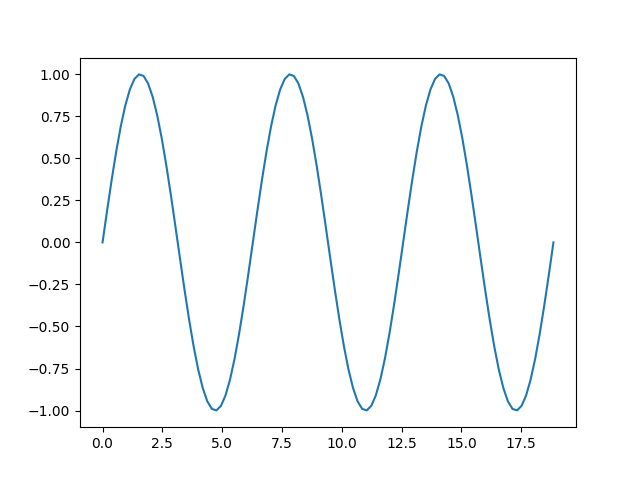
numpy的應用3+matplot
import matplotlib
import matplotlib.pyplot as plt
matplotlib.use("Agg")
import numpy as np
x = np.linspace(0,6*np.pi,100)
y = np.sin(x)
plt.plot(x,y)
plt.savefig("sinx.png")
print ('plot is done')
-
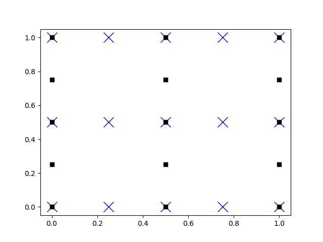
numpy的應用4+meshgrid+matplot
import numpy as np
import matplotlib.pyplot as plt
m, n = (5, 3)
x = np.linspace(0, 1, m)
y = np.linspace(0, 1, n)
X, Y = np.meshgrid(x,y)
print(x);print(y)
print(X);print(Y)
print(X.shape);print(Y.shape)
plt.plot(X, Y, 'bx', ms=15)
plt.plot(Y, X, 'ks')
plt.savefig("npmeshgrid.png")
print ('plot is done')
============output=============
[0.   0.25 0.5  0.75 1.  ]
[0.  0.5 1. ]
[[0.   0.25 0.5  0.75 1.  ]
 [0.   0.25 0.5  0.75 1.  ]
 [0.   0.25 0.5  0.75 1.  ]]
[[0.  0.  0.  0.  0. ]
 [0.5 0.5 0.5 0.5 0.5]
 [1.  1.  1.  1.  1. ]]
(3, 5)
(3, 5)
plot is done
-
numpy的應用5+matplot 3D
import matplotlib
import matplotlib.pyplot as plt
matplotlib.use("Agg")
import numpy as np

x1 = np.linspace(-2,2,5)
print ('x1=',x1)
x2=np.mgrid[-2:2:5j]
print ('x2=',x2)

x,y=np.mgrid[-2:2:5j,-2:2:5j]
print ('x=',x)
print ('y=',y)

x,y=np.mgrid[-2:2:10j,-2:2:10j]
plt.axis("equal")
plt.plot(x,y,'bo')
plt.savefig("5x5.png")

z=x**2+y**2
z2=x*0+y*0
from mpl_toolkits.mplot3d import Axes3D
fig = plt.figure()
ax = fig.gca(projection='3d')
ax.plot_surface(x, y, z, color="g")
ax.plot_surface(x, y, z2, color="b")
ax.scatter(0,0,0, color="k")
plt.savefig("mgrid-3D-1.png")
print ('plot is done')