用差分近似解微分方程式
-
數值積分(Numerical Integration)
首先讓我們來練習利用python程式寫一個積分的運算。 -
差分近似
差分近似: 考慮一個一階微分方程式: \[ \frac{dy}{dx}=f(x) , 初始值y(0)=1, f(x)是y的導函數 \] 如果y函數的一次導數就是他自己本身,那麼這個函數當然就是指數函數(\(\frac{d}{dx}e^x=e^x\)): \[f(x)=y, \rightarrow \frac{dy}{dx}=y \] \[\frac{dy}{y}=dx\] 兩邊積分可得 \[ \ln y=x \rightarrow 精確解:y(x)=e^{x} \] 差分近似的精神在於dx不是無窮小,只是很小,\[ dx=h\] \[ y(x+h) \simeq y(x)+ f(x)h \] \[ y(x+h) \simeq y(x)+ yh \] 從一個初始值開始可以用遞迴的方法把值向前推進,並且得到相對應的y,也就得到了我們微分方程的數值解。以這個方式獲得微分方成的數值解,我們稱之為Euler method。
-
Runge-Kutta 2nd order(RK2) method
-
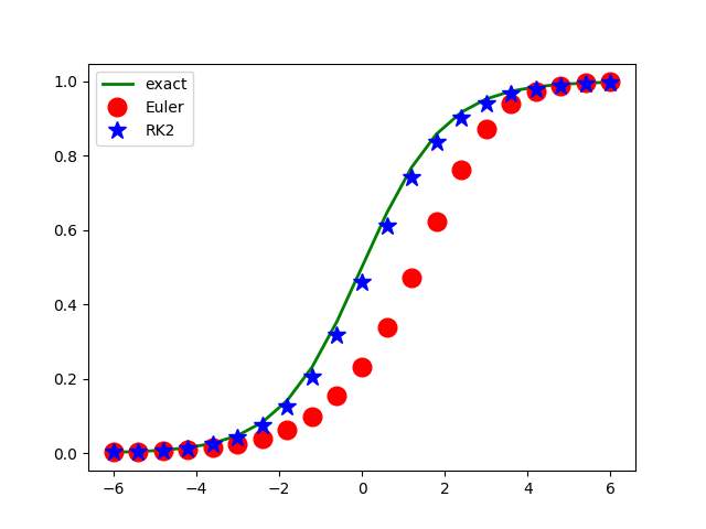
Logistic function
降落傘
一個降落傘從高空墜落時期運動方程式滿足下列的微分方程:\[ m\frac{dv}{dt}=mg-bv^2, v(0)=0 \] 其精確解為 \[v(t)=v_0 \tanh\frac{t}{T}, v_0=\sqrt{\frac{mg}{b}}, T=\sqrt{m/(gb)} \]- NONSEPARABLE EXACT ODE\[ \frac{dy}{dx}+\left(1+\frac{y}{x}\right)=0 \] exact solution: \[ y(x)=\frac{1}{x} \left( C-\frac{x^2}{2}\right) \]
- isobaric ODE:\[ \frac{dy}{dx}=-\frac{x^2-y}{x} \] exact solution: \[y(x)=Cx-x^2\]
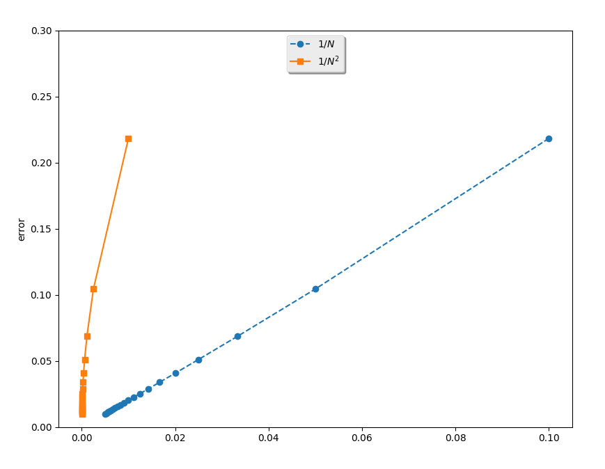
我們對一維積分做運算: \(\int\limits_a^b f(x)dx\)。先想好我們要將(a,b)的區域切割成多少(N)區間,那麼就可以根據上下限的距離(b-a)和分隔數(N),決定每一個區間的大小也就是\(dx=\frac{b-a}{N}\)。\[ \int\limits_a^b f(x)dx \simeq \sum\limits_{i=1}^N f(x_i) dx。\] 也就是用一個有限的級數求和來取代無窮的連續積分。
import matplotlib.pyplot as plt
import numpy as np

N=10
dt=np.pi/N
sum=0.
for i in range(N):
    t=dt*i
    sum+=dt*np.sin(t)
exact=2.
print ('num-integ=',sum,' exact=',exact)
error=abs(sum-exact)
print (N,error)
import numpy as np
import matplotlib.pyplot as plt

def f(x):
    y=np.sin(x)
    return y

def integrate(f, a, b, N):
    x = np.linspace(a, b, N)
    fx = f(x)
    area = np.sum(fx)*(b-a)/N
    return area

Er=[]
N1=[]
N2=[]
exact=2.
a,b=0,np.pi
print ('%6s %10s %10s' %('N','I','error'))
print ('---------------------------------')
for i in range(20):
    N=10*(i+1)
    N1.append(1./N)
    N2.append(1./N**2)
    I=integrate(f,a,b,N)
    error=np.abs(I-exact)
    Er.append(error)
    print ('%6d %10f.6 %10f.6' %(N,I,error))
#--------------------------------plot firgure with matplot
plt.plot(N1,Er,'--o',label='$1/N$')
plt.plot(N2,Er,'-s',label='$1/N^2$')
plt.legend(loc='upper center', shadow=True)
plt.ylabel('error')
plt.ylim(0,0.3)
plt.show()
     N          I      error
---------------------------------
    10   1.781686.6   0.218314.6
    20   1.895669.6   0.104331.6
    30   1.931442.6   0.068558.6
    40   1.948945.6   0.051055.6
    50   1.959329.6   0.040671.6
    60   1.966202.6   0.033798.6
    70   1.971088.6   0.028912.6
    80   1.974740.6   0.025260.6
    90   1.977572.6   0.022428.6
   100   1.979834.6   0.020166.6
   110   1.981681.6   0.018319.6
   120   1.983218.6   0.016782.6
   130   1.984517.6   0.015483.6
   140   1.985630.6   0.014370.6
   150   1.986593.6   0.013407.6
   160   1.987435.6   0.012565.6
   170   1.988178.6   0.011822.6
   180   1.988838.6   0.011162.6
   190   1.989428.6   0.010572.6
   200   1.989959.6   0.010041.6
import numpy as np
N=10
a,b=0.,1.
dt=(b-a)/N
t,x=a,1.
print ('%8s %8s %8s ' %('t','x','xe'))
print '---------------------------------'
for i in range(N+1):
    xe=np.exp(t)
    print ('%8.5f %8.5f %8.5f ' %(t,x,xe))
    t+=dt
    #------Euler
    x+=x*dt
       t       x1       xe
---------------------------------
 0.00000  1.00000  1.00000
 0.10000  1.10000  1.10517
 0.20000  1.21000  1.22140
 0.30000  1.33100  1.34986
 0.40000  1.46410  1.49182
 0.50000  1.61051  1.64872
 0.60000  1.77156  1.82212
 0.70000  1.94872  2.01375
 0.80000  2.14359  2.22554
 0.90000  2.35795  2.45960
 1.00000  2.59374  2.71828
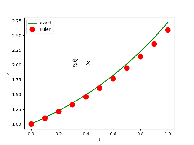
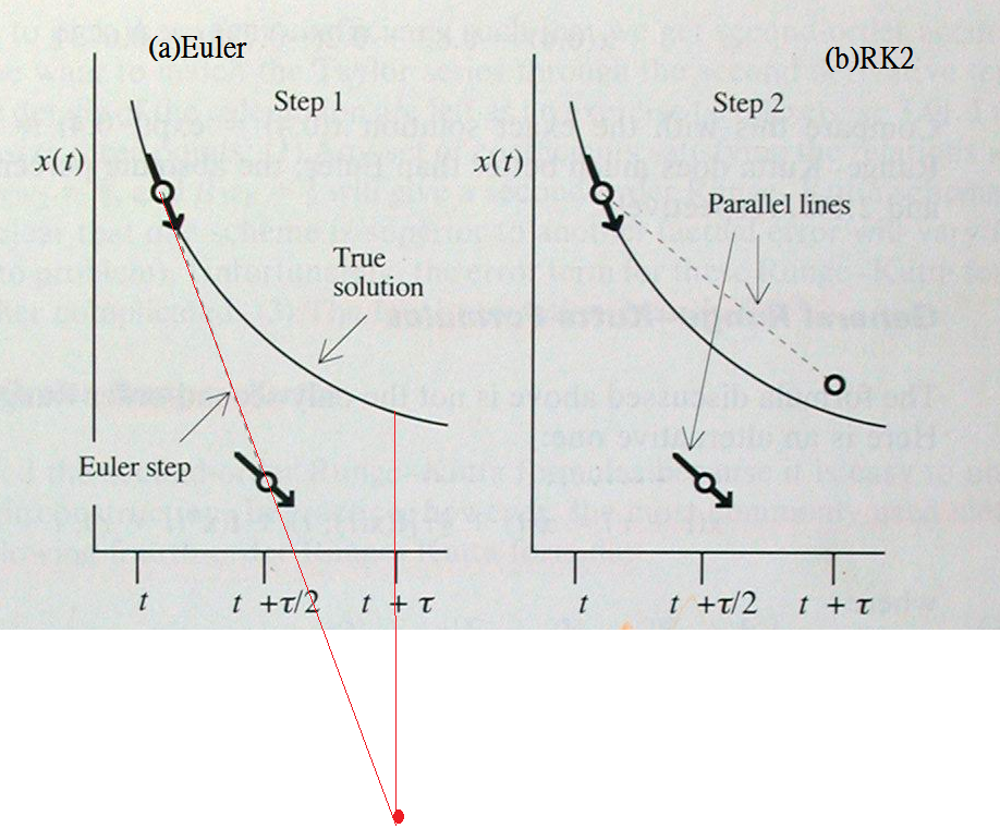
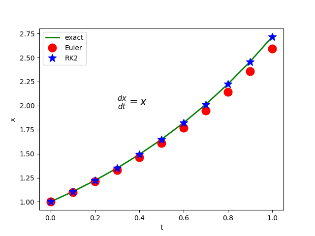
在下面的程式中我們同時使用Euler method和RK2來計算之前的微分方程式: \[ \frac{dx}{dt}=f(x,t)=x, x(0)=1\] 我們可以看見RK2的精確度1比Euler method高出許多。
import matplotlib.pyplot as plt
import numpy as np

def f(t,x):
    y=x
    return y

def exact(t):
    y=np.exp(t)
    return y

tp=[]; xep=[]; x1p=[]; x2p=[]
N=10
a,b=0.,1.
dt=(b-a)/N
t,x1,x2=a,1.,1.
print ('%8s %8s %8s %8s ' %('t','x1','x2','xe'))
print ('----------------------------------------')
for i in range(N+1):
    xe=exact(t)
    tp.append(t)
    xep.append(xe)
    x1p.append(x1)
    x2p.append(x2)
    print ('%8.5f %8.5f %8.5f %8.5f ' %(t,x1,x2,xe))
    #------Euler
    f1=f(t,x1)
    x1+=dt*f1
    #-------RK2
    f1=f(t,x2)
    xs=x2+(dt/2.)*f1
    ts=t+dt/2.
    f2=f(ts,xs)
    x2+=dt*f2
    t+=dt

plt.plot(tp, xep, color='green', label='exact',linestyle='solid',linewidth=2)
plt.plot(tp, x1p, 'o', color='red',label='Euler', markersize=12)
plt.plot(tp, x2p, '*', color='blue',label='RK2', markersize=12)
plt.xlabel('t')
plt.ylabel('x')
plt.title(r'$\frac{dx}{dt}=f(x,t)$'+'\n'+r'$f(x,t)=x$',  fontsize=15)
plt.legend()
plt.show()
       t       x1       x2       xe
----------------------------------------
 0.00000  1.00000  1.00000  1.00000
 0.10000  1.10000  1.10500  1.10517
 0.20000  1.21000  1.22103  1.22140
 0.30000  1.33100  1.34923  1.34986
 0.40000  1.46410  1.49090  1.49182
 0.50000  1.61051  1.64745  1.64872
 0.60000  1.77156  1.82043  1.82212
 0.70000  1.94872  2.01157  2.01375
 0.80000  2.14359  2.22279  2.22554
 0.90000  2.35795  2.45618  2.45960
 1.00000  2.59374  2.71408  2.71828

import matplotlib.pyplot as plt
import numpy as np

def f(t,x):
    y=x*(1.-x)
    return y

def exact(t):
    y=1./(1.+np.exp(-t))
    return y

tp=[]; xep=[]; x1p=[]; x2p=[]
N=20
a,b=-6.,6.
dt=(b-a)/N
t,x1,x2=a,np.exp(a),np.exp(a)
print ('%8s %8s %8s %8s ' %('t','x1','x2','xe'))
print ('----------------------------------------')
for i in range(N+1):
    xe=exact(t)
    tp.append(t)
    xep.append(xe)
    x1p.append(x1)
    x2p.append(x2)
    print ('%8.5f %8.5f %8.5f %8.5f ' %(t,x1,x2,xe))
    #------Euler
    f1=f(t,x1)
    x1+=dt*f1
    #-------RK2
    f1=f(t,x2)
    xs=x2+(dt/2.)*f1
    ts=t+dt/2.
    f2=f(ts,xs)
    x2+=dt*f2
    t+=dt

plt.plot(tp, xep, color='green', label='exact',linestyle='solid',linewidth=2)
plt.plot(tp, x1p, 'o', color='red',label='Euler', markersize=12)
plt.plot(tp, x2p, '*', color='blue',label='RK2', markersize=12)
plt.xlabel('t')
plt.ylabel('x')
plt.title(r'$\frac{dx}{dt}=f(x,t)$'+'\n'+r'$f(x,t)=x(1-x)$',  fontsize=15)
plt.legend()
plt.show()
       t       x1       x2       xe
----------------------------------------
-6.00000  0.00248  0.00248  0.00247
-5.40000  0.00396  0.00440  0.00450
-4.80000  0.00633  0.00782  0.00816
-4.20000  0.01010  0.01384  0.01477
-3.60000  0.01611  0.02441  0.02660
-3.00000  0.02561  0.04275  0.04743
-2.40000  0.04059  0.07395  0.08317
-1.80000  0.06395  0.12528  0.14185
-1.20000  0.09987  0.20517  0.23148
-0.60000  0.15381  0.31889  0.35434
-0.00000  0.23190  0.46082  0.50000
 0.60000  0.33877  0.61007  0.64566
 1.20000  0.47318  0.74032  0.76852
 1.80000  0.62274  0.83704  0.85815
 2.40000  0.76370  0.90133  0.91683
 3.00000  0.87198  0.94141  0.95257
 3.60000  0.93896  0.96558  0.97340
 4.20000  0.97335  0.97989  0.98523
 4.80000  0.98891  0.98829  0.99184
 5.40000  0.99549  0.99319  0.99550
 6.00000  0.99818  0.99605  0.99753