-
:高斯消去法
-
使用numpy的linalg函數求解方程式
-
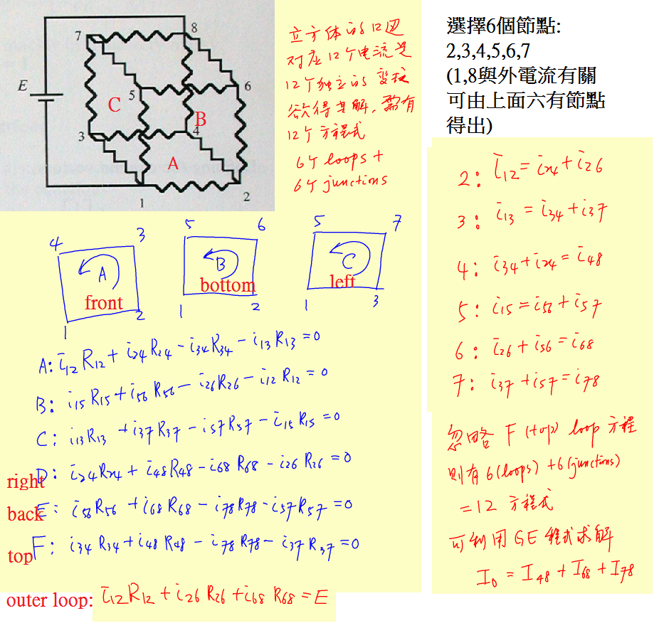
Resistors network; KCL/KVL
-
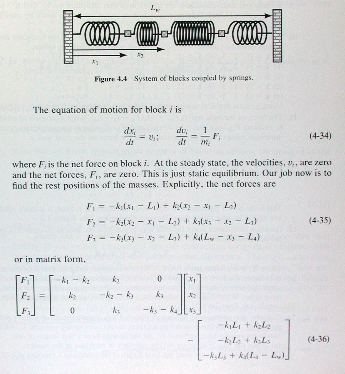
coupled springs
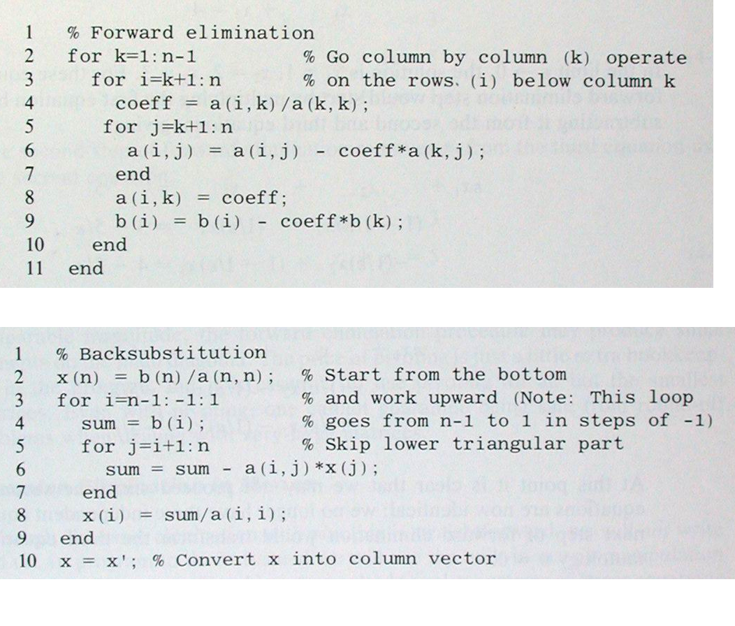
線性代數1:高斯消去法解方程組
In order to get acquainted with the matrix calculations in python, you can refer to the following web site: Python--線性代數篇(numpy)
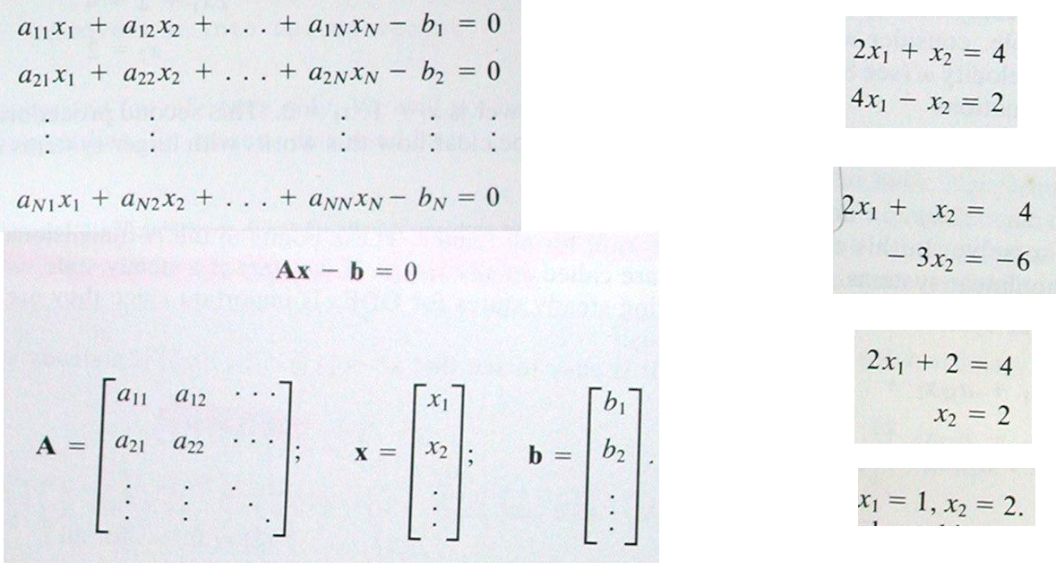
There are very useful functions in numpy for us to solve linear system of equations. Use the following statement you can get the solutions (x) for the matrix equation:\( \mathbf{A} x= b\)
x = np.linalg.solve(A, b)
import numpy as np A = np.array([[3,1], [1,2]]) b = np.array([9,8])x = np.linalg.solve(A, b) #解聯立方程式 print x print np.allclose(np.dot(A, x), b)
import numpy as np A = np.array([[3,2,1], [2,3,1], [1,1,4]]) b = np.array([11,13,12])x = np.linalg.solve(A, b) print x print np.allclose(np.dot(A, x), b)
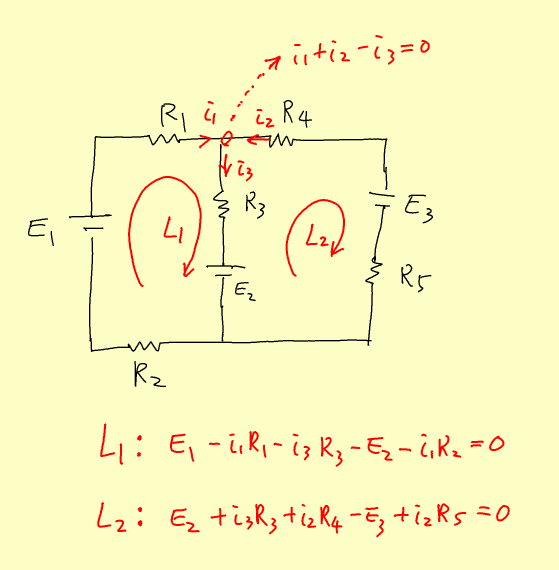
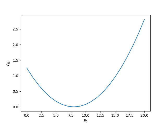
\[ i_1+i_2-i_3=0\] \[-(R_1 + R_2)i_1 -R_3i_3=E_2-E_1 \] \[-(R_4+R_5)i_2 -R_3 i_3 = E_2-E_3 \] Take the following values: \[ R_1=R_2=1, R_3=R_4=2, R_5=5, E_1=2, E_3=5 \] \(E_2\) is a variable :\[ 0 \lt E_2 \lt 20 \] Calculate the power of \(R_5\) as a function of the voltage \(E_2\).
import numpy as np
import matplotlib.pyplot as plt
R1=1.; R2=1.; R3=2.; R4=2.; R5=5.; E1=2.; E3=5.
E=[]; p5=[]
for i in range(21):
    E2=0.+1.*i
    a = np.array([[1,1,-1], [-(R1+R2),0,-R3], [0,-(R4+R5),-R3]])
    b = np.array([0,E2-E1,E2-E3])
    x = np.linalg.solve(a, b)
    power5=x[1]**2*R5
    print E2,power5
    E.append(E2)
    p5.append(power5)
plt.plot(E,p5)
plt.show()
\( \begin{aligned} a & = b & (1) \\ c & = d & (2) \end{aligned} \)
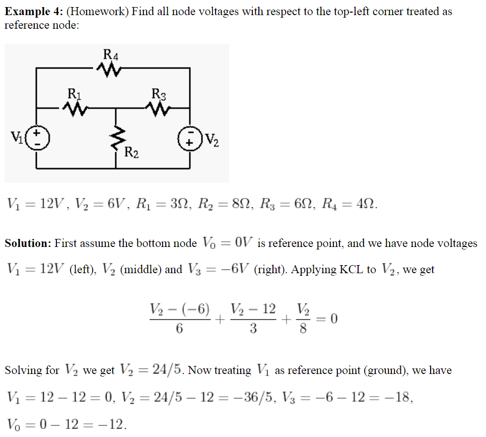
\(\begin{aligned} i_1+i_4-i_5 &= 0 & (1) \\ i_1-i_2-i_3 &= 0 & (2) \\ i_3+i_4-i_6 &= 0 & (3) \\ i_2-i_5+i_6 &= 0 & (4) \\ R_1i_1+R_2i_2 &= V_1 & (5) \\ -R_2i_2+R_3i_3 &= V_2 & (6) \\ R_1i_1+R_3i_3-R_4i_4 &= 0 & (7) \end{aligned} \)
Take the following values: \[ R_1=3; R_2=8; R_3=6; R_4=4; V_1=12; V_2=6 \] Solve the equations and get all currents. There are 7 equations and 6 variables, you can neglect eqn.(4).
import numpy as np
import matplotlib.pyplot as plt
def cube(R57):
R12=1.
R13=1.
R15=1.
R24=1.
R26=1.
R34=1.
R37=1.
R48=1.
R56=1.
#R57=1.
R68=1.
R78=1.
E=1.
N=12
a1=[]; b1=[]
for i in range(N):
b1.append(0.)
row=[]
for j in range(N):
row.append(0.)
a1.append(row)
a = np.asarray(a1)
b = np.asarray(b1)
b[5]=E
a[0][0]=R12; a[0][3]=R24; a[0][5]=-R34; a[0][1]=-R13
a[1][2]=R15; a[1][8]=R56; a[1][4]=-R26; a[1][0]=-R12
a[2][1]=R13; a[2][6]=R37; a[2][9]=-R57; a[2][2]=-R15
a[3][3]=R24; a[3][7]=R48; a[3][10]=-R68; a[3][4]=-R26
a[4][8]=R56; a[4][10]=R68; a[4][11]=-R78; a[4][9]=-R57
a[5][0]=R12; a[5][4]=R26; a[5][10]=R68
a[6][0]=1.; a[6][3]=-1.; a[6][4]=-1.
a[7][1]=1.; a[7][5]=-1.; a[7][6]=-1.
a[8][5]=1.; a[8][3]=1.; a[8][7]=-1.
a[9][2]=1.; a[9][8]=-1.; a[9][9]=-1.
a[10][4]=1.; a[10][8]=1.; a[10][10]=-1.
a[11][6]=1.; a[11][9]=1.; a[11][11]=-1.
return a,b
R=[]; r57=[]
for i in range(21):
R57=0.+0.1*i
r57.append(R57)
a,b=cube(R57)
x = np.linalg.solve(a, b)
Io=x[7]+x[10]+x[11]
Req=1./Io
R.append(Req)
print R57,Req
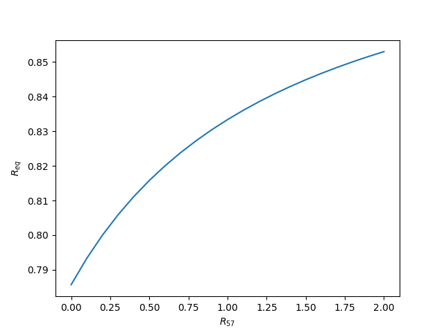
plt.plot(r57,R)
plt.xlabel('$R_{57}$')
plt.ylabel('$R_{eq}$')
plt.show()
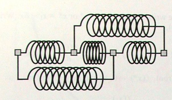
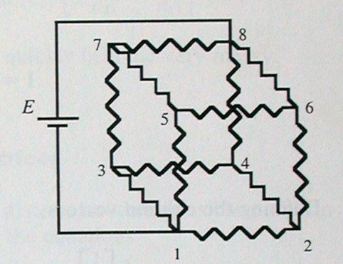
resistors cube-2