計算物理

利用numpy函數做數據的統計分析

numpy是一個非常有用的數值計算工具，在這個講次中我們先簡單介紹如何利用numpy函數做數據的統計分析。

陣列的內建函數

NumPy矩陣本身在初始化之後就內建一些好用的方法！

sum：矩陣加總
min：矩陣最小值
max：矩陣最大值
mean：矩陣平均值
sum(axis=1)：指定要加總的矩陣維度
cumsum()：累計加總
random.seed()：設定亂數的種子，以這個種子為開端產生的亂數序列都相同。
np.random.random((12))：產生12個亂數的一維陣列。
round(a,2)：將a陣列中的所有浮點數四捨五入至小數點第2位

import matplotlib
matplotlib.use("Agg")
import matplotlib.pyplot as plt
import numpy as np

a = np.random.random((3, 3))
print('a=\n',a)
a1=a.sum()
a2=a.max()
a3=a.min()
a4=a.mean()
print('a.sum()=',a1)
print('a.max()=',a2)
print('a.min()=',a3)
print('a.mean()=',a4,a4*9)

b = np.arange(12).reshape(2, 6)
print('\nb=\n',b)
print('b.sum(axis=0)=',b.sum(axis=0))
print('b.sum(axis=1)=',b.sum(axis=1))

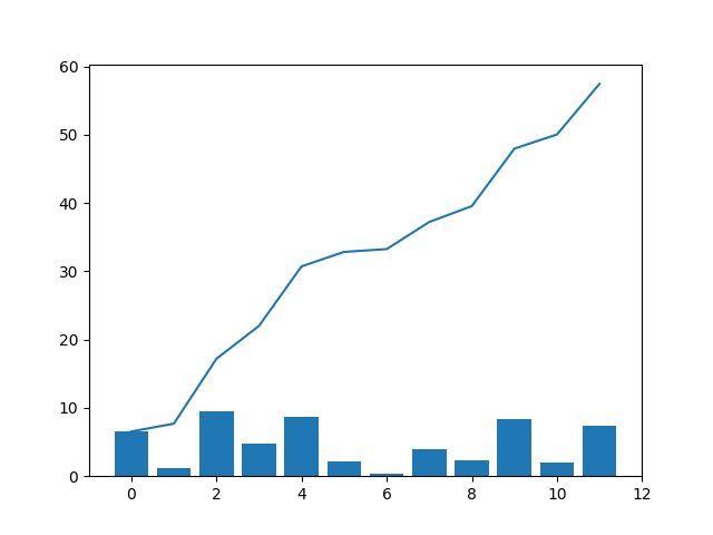
np.random.seed(1000)
revenu = np.round(np.random.random((12)) * 10., 2)
x=np.arange(0,len(revenu),1)
print('revenu=',revenu)
revcum=revenu.cumsum()
print('Cumulative Sum of revenu=\n',revcum)
plt.bar(x,revenu)
plt.plot(x,revcum)
plt.savefig("np-arr-func.png")

============輸出:=============

a=
 [[0.39215413 0.18225652 0.74353941]
 [0.06958208 0.8853372  0.9526444 ]
 [0.93114343 0.41543095 0.02898166]]
a.sum()= 4.601069794034902
a.max()= 0.9526443992215418
a.min()= 0.02898165938687125
a.mean()= 0.5112299771149891 4.601069794034902
b=
 [[ 0  1  2  3  4  5]
 [ 6  7  8  9 10 11]]
b.sum(axis=0)= [ 6  8 10 12 14 16]
b.sum(axis=1)= [15 51]
revenu= [6.54 1.15 9.5  4.82 8.72 2.12 0.41 3.97 2.33 8.42 2.07 7.42]
Cumulative Sum of revenu=
 [ 6.54  7.69 17.19 22.01 30.73 32.85 33.26 37.23 39.56 47.98 50.05 57.47]

一維數據的簡易統計分析

這個程式中我們展現簡單的一維數據的統計分析我們用到的函數包括：

np.mean(a)：全體數據的平均值
np.var(a)：全體數據地方差
np.std(a)：全體數據的標準差
np.median(a)：全體數據的中位數
np.average(a,weights=wts,returned=True)：weights=wts，數據依照wts權重值陣列作權重平均。returned=True，回傳權重的總和。
np.histogram(bins[1:],hist)：依照bins陣列所定義的分隔，計算a陣列中在各分隔區中的數量hist。

import matplotlib
matplotlib.use("Agg")
import matplotlib.pyplot as plt
import numpy as np

a = np.array([1,  2,  3,  4])
mean_a=np.mean(a)
var_a=np.var(a)
std_a=np.std(a)
print('a=',a)
print ('np.mean(a)=',mean_a)

s=0.
for i in range(4):
    s+=(a[i]-mean_a)**2
s=s/4.

print ('np.var(a)=',var_a,s)
print ('np.std(a)=',std_a,np.sqrt(s))

print('median=',np.median(a))
wts=[2.,1.,2.,1.]
print(a)
print(wts)
print('weighted average=',np.average(a,weights = wts, returned =  True))

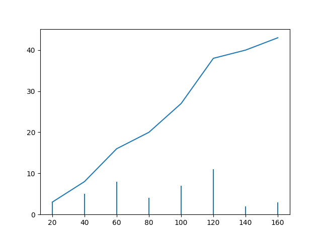
a = np.array([22,87,5,43,56,73,55,54,11,20,51,5,79,31,27])
np.histogram(a,bins =  [0,20,40,60,80,100])
hist,bins = np.histogram(a,bins =  [0,20,40,60,80,100])
print (hist)
print (bins[1:])
plt.bar(bins[1:],hist)
plt.savefig("np-statistics.png")
print('plot is done.')

============輸出:=============

a= [1 2 3 4]
np.mean(a)= 2.5
np.var(a)= 1.25 1.25
np.std(a)= 1.118033988749895 1.118033988749895
median= 2.5
[1 2 3 4]
[2.0, 1.0, 2.0, 1.0]
weighted average= (2.3333333333333335, 6.0)
[3 4 5 2 1]
[ 20  40  60  80 100]
plot is done.

3/16作業題目

首先請你把這個a陣列切出3個不同的一維陣列分別叫做b0,b1,b2。對於b1一維陣列，也就是對應到各科目的選課人數，請你先找出b1的最大值、最小值、平均值、總和、方差、標準差和中位數。

接著請你建立下面這個一維陣列bins=[0,20,40,60,80,100,120,140,160]，這個陣列的目的是要把選修學生人數切分為0到20，20到40，40到60，等等，然後統計每一科目的選修學生人數落在每一個分隔當中的科目數量(hist)。然後再獲取所有分隔人數的累積數量(histcum)。

利用bins,hist,histcum這三個一維陣列的數據，可以畫出下面的科目數量對選修學生人數的分佈圖

利用b2的數據把科目區分為1類和2類，也就是生命科學類(1_和非生命科學類(2)，收集這些類別當中的科目代號，然後把它們依據類別列印出科目代號，並且計算在生命科學領域中的科目數目和選修這個領域的所有學生人總數，以及同樣的計算非生命科學領域的科目的數量以及選修非生命科學領域的學生總數。

最後請你以b2為權重函數，以這個陣列來對學生人數b1進行權重平均。

a=np.array([[3081,3082,	3083,3084,3085,	3086,3087,3088,3089,3090,
3092,3093,3094,3096,3098,3099,3100,3101,3102,3104,3105,	3106,
3107,3108,3109,3110,3112,3113,3114,3115,3116,3117,3118,3119,
3120,3121,3122,3123,3124,3125,3126,8611,8612],[49,23,17,57,
35,35,89,102,45,107,106,59,159,74,125,127,89,85,60,114,	
118,81,77,28,54,54,110,98,107,150,111,109,107,81,150,55,	
58,17,32,6,75,86,107], [2,2,2,2,2,2,1,2,2,1,1,2,1,2,	
2,2,2,2,2,1,1,1,1,1,1,1,1,1,1,1,1,1,1,1,1,2,1,1,	
1,2,2,2,1]])
print('a=\n',a)
print(np.shape(a))